Piecewise Functions: The Hidden Framework of Modern Deep Learning

Introduction: The Power of Breaking Things Apart

Have you ever wondered why neural networks can approximate any continuous function? Or why modern deep learning works so well in practice? The answer lies in a fundamental mathematical concept: piecewise functions.

The name “Piecewise” represents more than just a mathematical construct—it embodies a powerful principle in science and engineering: complex problems can be solved by breaking them into simpler, manageable pieces.

Mathematical Foundations

What Makes a Function Piecewise?

A piecewise function is formally defined as:

where ({I_1, I_2, \dots, I_n}) forms a partition of the domain. Each (I_k) is called a “piece” of the domain, and (f_k) is the function defined on that piece.

The Beauty of Discontinuity

Not all piecewise functions are created equal. Let’s explore three levels of regularity:

1. Discontinuous Piecewise Functions
   • Classic example: The Heaviside function
   \[H(x) = \begin{cases} 0 & \text{if } x < 0 \\ 1 & \text{if } x \geq 0 \end{cases}\]

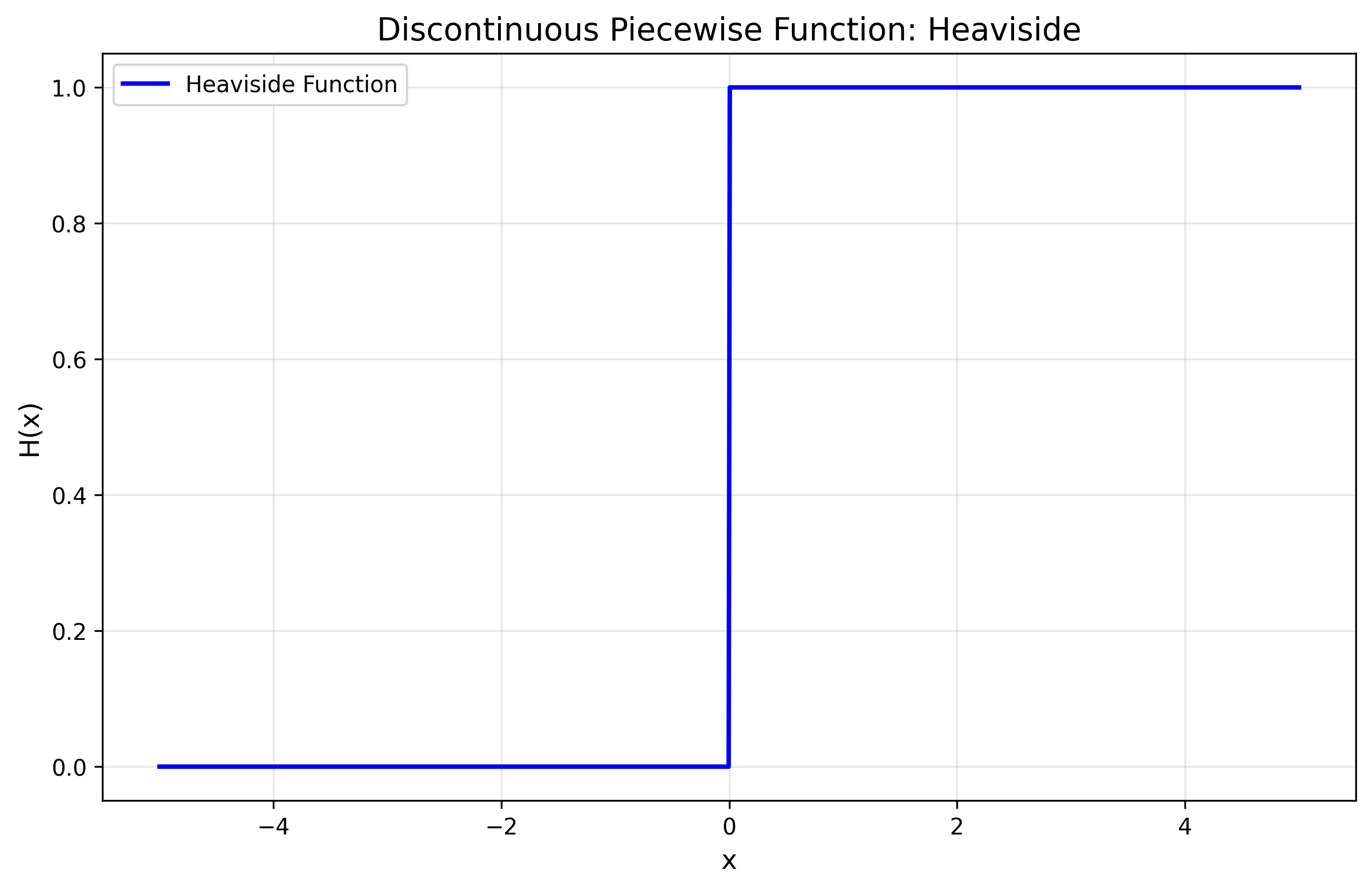   Figure 1: The Heaviside function demonstrating discontinuous behavior at x = 0

   • Applications:
     • Digital signal processing (step responses)
     • Quantum mechanics (potential wells)
     • Control systems (bang-bang control)
2. Continuous Piecewise Functions
   • The famous ReLU function:
   \[\text{ReLU}(x) = \max(0, x) = \begin{cases} 0 & \text{if } x < 0 \\ x & \text{if } x \geq 0 \end{cases}\]

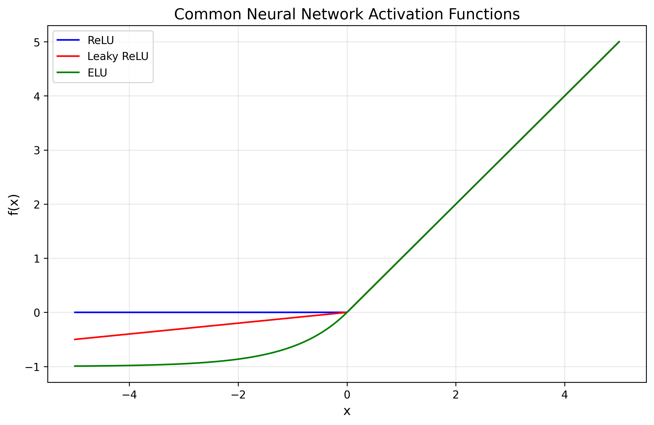Figure 2: Common neural network activation functions

 - Properties:
   - Continuous everywhere
   - Not differentiable at \( x = 0 \)
   - Linear behavior in the positive regime

1. Smooth Piecewise Functions
   • Cubic splines with mathematical form:
   \[S_i(x) = a_i(x - x_i)^3 + b_i(x - x_i)^2 + c_i(x - x_i) + d_i\]

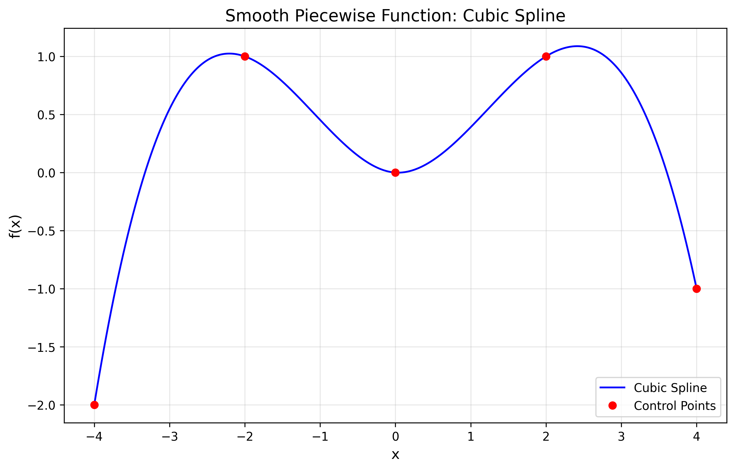Figure 4: A cubic spline showing smooth piecewise behavior

• Properties:
  • Continuous up to the second derivative
  • Natural interpolation
  • Minimal curvature property

The Deep Learning Connection

ReLU: The Building Block of Modern Neural Networks

The Rectified Linear Unit (ReLU) is perhaps the most important piecewise function in modern machine learning. Its simplicity belies its power:

import numpy as np
def relu(x):
    return np.maximum(0, x)

# Vectorized implementation
def relu_vectorized(X):
    return np.maximum(0, X)

What Makes ReLU Special? Let’s Analyze its Properties

Sparsity

Mathematical representation:

• Creates naturally sparse representations
• Helps in feature selection

Non-Saturation

Gradient behavior:

• No vanishing gradient for positive inputs

Universal Approximation: The Theory

The Universal Approximation Theorem makes a profound statement about neural networks with piecewise activation functions. For any continuous function ( f: [a, b] \rightarrow \mathbb{R} ) and ( \epsilon > 0 ), there exists a neural network ( N ) with ReLU activations such that:

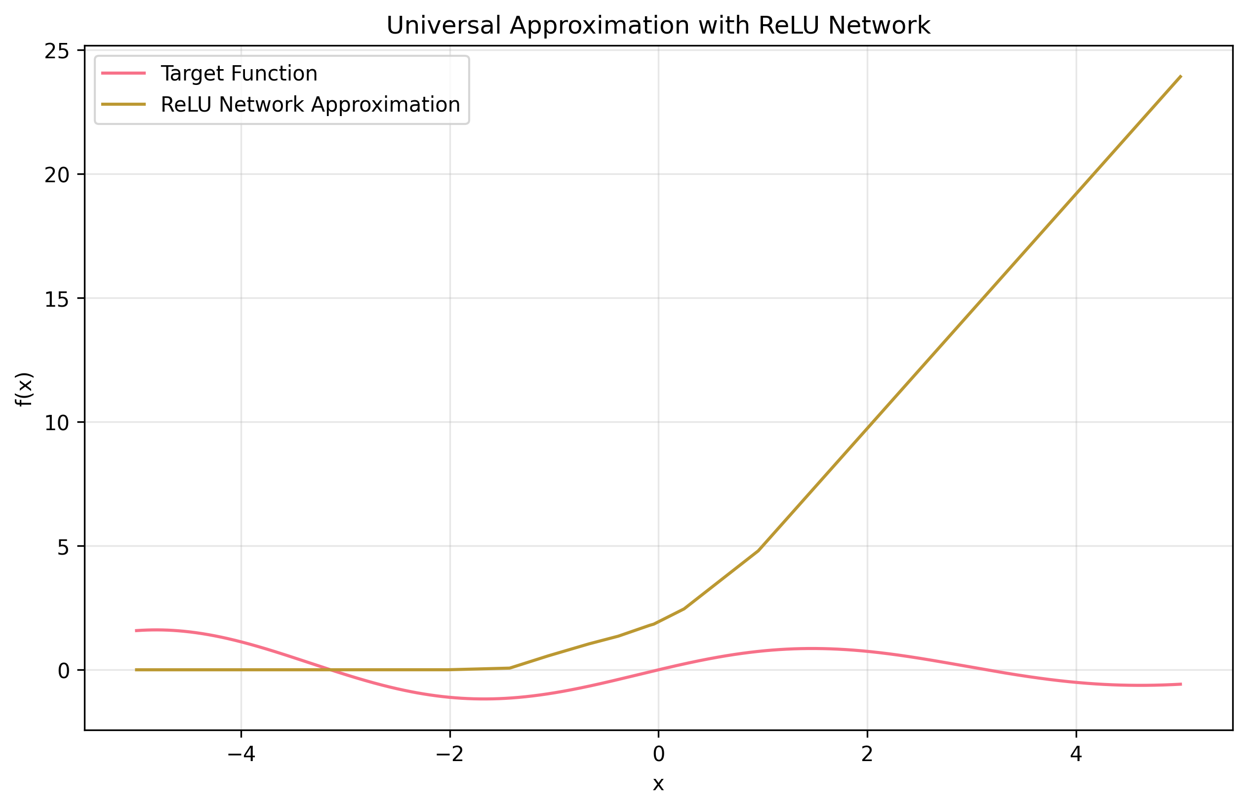Figure 3: Example of universal approximation using ReLU networks

This is achieved through:

1. Local Linear Approximation

   Each ReLU unit contributes a “hinge”:

   \[h_i(x) = \max(0, w_i x + b_i)\]

2. Composition of Pieces

   Network output:

   \[N(x) = \sum_{i=1}^n v_i \max(0, w_i x + b_i)\]

Practical Applications

Let’s implement some key concepts in Python:

import numpy as np
import matplotlib.pyplot as plt

# Different activation functions
def relu(x): 
    return np.maximum(0, x)

def leaky_relu(x, alpha=0.01): 
    return np.where(x > 0, x, alpha * x)

def elu(x, alpha=1.0): 
    return np.where(x > 0, x, alpha * (np.exp(x) - 1))

# Visualization
x = np.linspace(-5, 5, 1000)
functions = {
    'ReLU': relu(x),
    'Leaky ReLU': leaky_relu(x),
    'ELU': elu(x)
}

plt.figure(figsize=(12, 6))
for name, f in functions.items():
    plt.plot(x, f, label=name)
plt.grid(True)
plt.legend()
plt.title('Common Neural Network Activation Functions')
plt.xlabel('x')
plt.ylabel('f(x)')
plt.show()

Future Directions

The story of piecewise functions continues to evolve:

• Theoretical Developments
  • New activation function designs
  • Improved approximation theorems
  • Connections to geometric deep learning
• Practical Applications
  • Hardware-efficient implementations
  • Sparse computation methods
  • Automated architecture design

Conclusion

The principle of piecewise decomposition extends beyond mathematics—it’s a fundamental way of understanding complexity. By breaking down complex problems into simpler, manageable pieces, we can:

• Build intuitive understanding
• Develop efficient algorithms
• Create scalable solutions

This is why I chose “Piecewise” as my portfolio name. It represents not just a mathematical concept, but a philosophy: complex problems become manageable when broken into pieces, just as complex functions become understandable through their piecewise representations.

References

• Glorot, X., et al. (2011). “Deep Sparse Rectifier Neural Networks”
• He, K., et al. (2015). “Delving Deep into Rectifiers”
• Cybenko, G. (1989). “Approximation by Superpositions of a Sigmoidal Function”
• Hornik, K. (1991). “Approximation Capabilities of Multilayer Feedforward Networks”

Note: This post assumes basic familiarity with calculus and neural networks. For a gentler introduction to these concepts, see my upcoming post on mathematical foundations of deep learning.